3. Prepare Fermi LAT data with gtselect and gtmktime

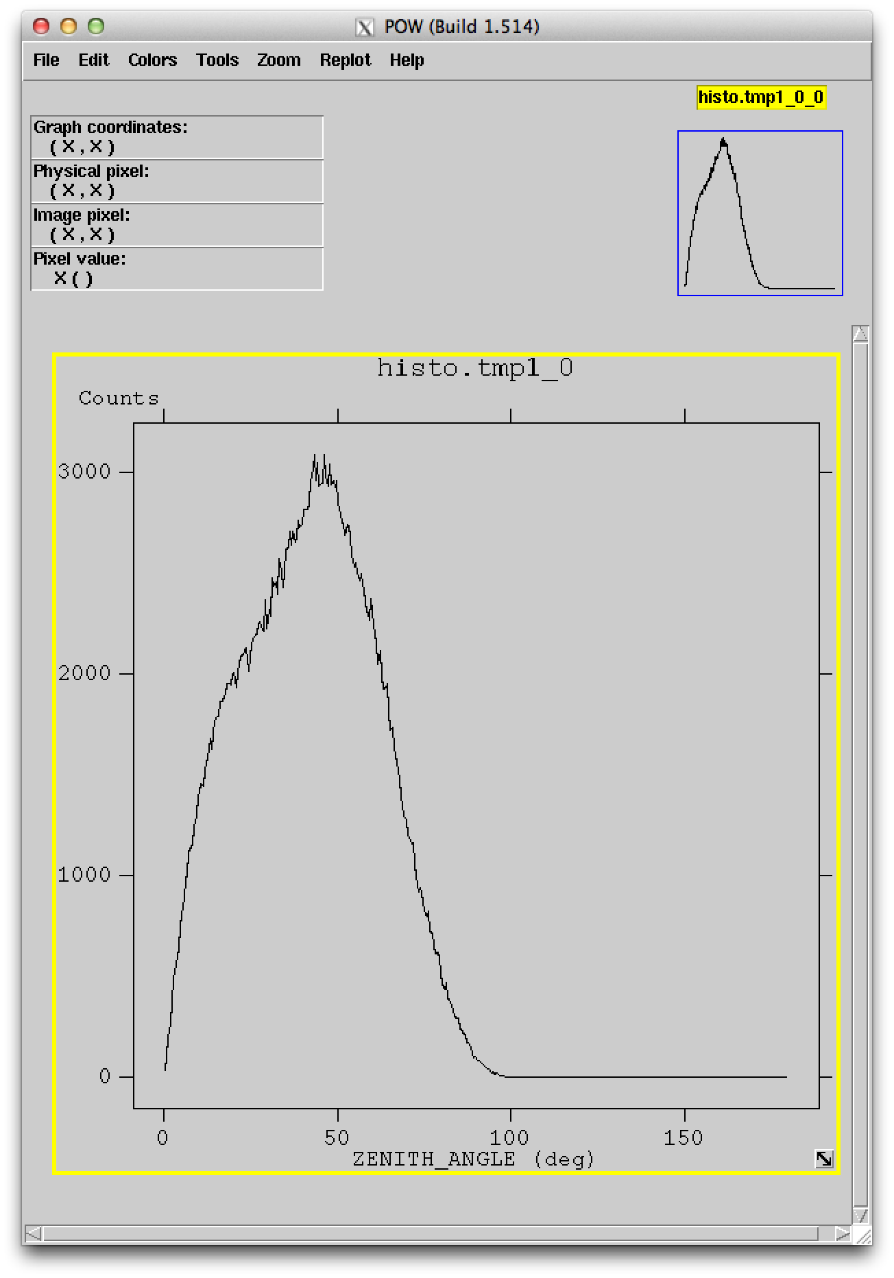
In the last section we made a histogram of the photon zenith angle distribution and found a broad peak in the range 0 to 100 deg and a narrow peak around 113 deg.

The narrow peak at a zenith angle of ~ 113 deg is due to “atmospheric gamma rays” as explained in the following Figure (which also explains what the zenith angle is).

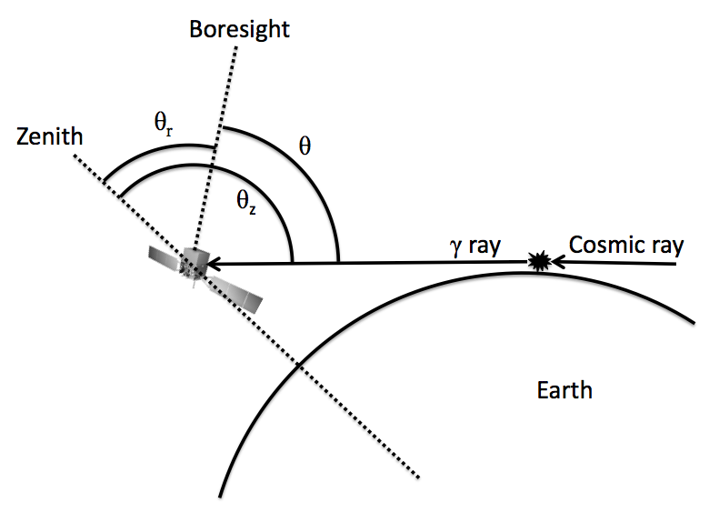
Schematic of Limb gamma-ray production by cosmic ray interactions in the Earth’s atmosphere, showing the definitions of the zenith angle (θz), the spacecraft rocking angle (θr) and the incidence angle (θ). Reference: http://adsabs.harvard.edu/abs/2013arXiv1305.5597F

We are not interested in atmospheric gamma rays, only in gamma rays from (non-atmospheric) astrophysical sources.

To apply selection cuts that remove the atmospheric gammas we will use the gtselect and gtmktime Fermi Science Tools (the Fermi LAT FTOOLS). Running these two tools has other purposes, too, e.g. selecting an event class (see LAT Data Selection Recommendations for more information).

We will not describe the details of what happens here ... if you are interested read the Fermi LAT Data Preparation analysis thread and follow the links given there.

gtselect takes an FITS event file as input and writes a subset of events to an output FITS event file. If you have more than one input FITS event file you have to create a text file containing the names of all FITS event files you’d like to process ... one file per line.

Use the command line ls utility to create the text file and the cat utility to print it’s contents to the terminal to check that it worked:

$ ls -1 *_PH??.fits > events.txt
$ cat events.txt
L1309081333300B976F4377_PH00.fits
L1309081333300B976F4377_PH01.fits

Now run gtselect and select event class 2, corresponding to P7SOURCE_V6, as well as a maximum zenith angle of 100 deg as recommended here:

$ gtselect evclass=2
Input FT1 file[] @events.txt
Output FT1 file[] gtselect.fits
RA for new search center (degrees) (0:360) [] INDEF
Dec for new search center (degrees) (-90:90) [] INDEF
radius of new search region (degrees) (0:180) [] INDEF
start time (MET in s) (0:) [] INDEF
end time (MET in s) (0:) [] INDEF
lower energy limit (MeV) (0:) [] 100
upper energy limit (MeV) (0:) [] 1000000
maximum zenith angle value (degrees) (0:180) [] 100
Done.

Note that we had to specify the evclass parameter on the command line, because it’s a hidden FTOOL parameter:

$ plist gtselect
Parameters for /Users/deil/pfiles/gtselect.par
       infile = @events.txt      Input FT1 file
      outfile = gtselect.fits    Output FT1 file
           ra = INDEF            RA for new search center (degrees)
          dec = INDEF            Dec for new search center (degrees)
          rad = INDEF            radius of new search region (degrees)
         tmin = INDEF            start time (MET in s)
         tmax = INDEF            end time (MET in s)
         emin = 100              lower energy limit (MeV)
         emax = 1000000          upper energy limit (MeV)
         zmax = 100              maximum zenith angle value (degrees)
    (evclsmin = INDEF)           Minimum event class ID
    (evclsmax = INDEF)           Maximum event class ID
     (evclass = 2)               Event class selection (e.g. 0=Transient, 2=Source)
    (convtype = -1)              Conversion type (-1=both, 0=Front, 1=Back)
    (phasemin = 0)               minimum pulse phase
    (phasemax = 1)               maximum pulse phase
     (evtable = EVENTS)          Event data extension
     (chatter = 2)               Output verbosity
     (clobber = yes)             Overwrite existing output files
       (debug = no)              Activate debugging mode
         (gui = no)              GUI mode activated
        (mode = ql)              Mode of automatic parameters

Sometimes it’s convenient to give the parameters on the command line to avoid the interactive prompt.

E.g. after you’ve done a few Fermi data analyses you’ll get tired of running the tools interactively and will want to use scripts where you substitute in the correct parameters in the correct places. Shell scripts, Makefiles or Python scripts are common choices.

Later in this tutorial you’ll use a set of easy-to-use Fermi LAT data analysis Python scripts called Enrico to do the busywork.

The following command is equivalent to the gtselect command given above ... you can simply copy & paste it in you terminal:

$ gtselect infile=@events.txt outfile=gtselect.fits \
  ra=INDEF dec=INDEF rad=INDEF tmin=INDEF tmax=INDEF \
  emin=100 emax=1000000 zmax=100 evclass=2

The backslash tells the terminal that the command is not finished and will continue on the next line.

Did you note how we used INDEF to denote “don’t apply an additional cut” for the region of interest (ROI) and the time range? INDEF doesn’t work for the energy range apparently, so we had to repeat the selection we made when downloading the data: 100 MeV to 1,000,000 MeV = 1 TeV.

If you ever forget what Data Sub Space (DSS) selections you applied when downloading the data or processing it with gtselect or gtmktime, you can use the gtvcut tool to display a summary:

$ gtvcut L1309081333300B976F4377_PH00.fits EVENTS
DSTYP1: TIME
DSUNI1: s
DSVAL1: TABLE
DSREF1: :GTI

GTIs: (suppressed)

DSTYP2: BIT_MASK(EVENT_CLASS,2)
DSUNI2: DIMENSIONLESS
DSVAL2: 1:1

DSTYP3: POS(RA,DEC)
DSUNI3: deg
DSVAL3: CIRCLE(83.633083,22.0145,20)

DSTYP4: TIME
DSUNI4: s
DSVAL4: 378691200:394329600

DSTYP5: ENERGY
DSUNI5: MeV
DSVAL5: 100:1000000

Back to business ... let’s finish the data preparation by running gtmktime using the recommended parameters from here:

$ gtmktime
Spacecraft data file[] ../spacecraft.fits
Filter expression[] DATA_QUAL==1&&LAT_CONFIG==1&&ABS(ROCK_ANGLE)<52
Apply ROI-based zenith angle cut[] yes
Event data file[] gtselect.fits
Output event file name[] gtmktime.fits

Note

For this tutorial I chose to name the gtselect tool output file gtselect.fits and the gtmktime output file gtmktime.fits. I find this convention of using the tool name as output file name easy to remember, but you can choose any file names you like of course.

Before moving on to the next section, which will explain a bit what gtselect and gtmktime have done, let’s use fv again to plot the ZENITH_ANGLE distribution of gtmktime.fits. As expected, there are no events with ZENITH_ANGLE > 100 deg any more.