3. Create count and and model images with the Fermi Science Tools

3.1. Make a count image with gtbin

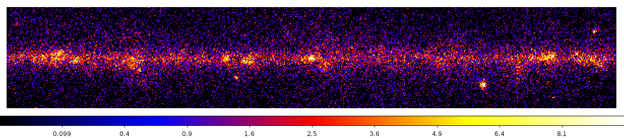
Run gtbin to make a counts image:

$ gtbin
This is gtbin version ScienceTools-v9r31p1-fssc-20130410
Type of output file (CCUBE|CMAP|LC|PHA1|PHA2|HEALPIX) [] CMAP
Event data file name[] gtmktime.fits
Output file name[] count_image.fits
Spacecraft data file name[] ../../spacecraft.fits
Size of the X axis in pixels[] 600
Size of the Y axis in pixels[] 100
Image scale (in degrees/pixel)[] 0.1
Coordinate system (CEL - celestial, GAL -galactic) (CEL|GAL) [] GAL
First coordinate of image center in degrees (RA or galactic l)[] 0
Second coordinate of image center in degrees (DEC or galactic b)[] 0
Rotation angle of image axis, in degrees[] 0
Projection method e.g. AIT|ARC|CAR|GLS|MER|NCP|SIN|STG|TAN:[] CAR

Open up the image in ds9 and use the following commands to get an image that looks like this:

• Select Scale -> Scale Parameters and sqrt with range 0 to 10.
• Color -> b

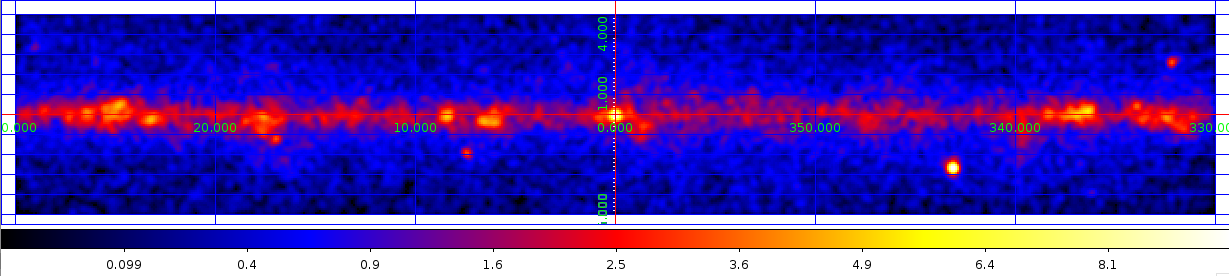
Now use these options to get the following view of the same counts image:

• Analysis -> Smooth Parameters with a 3 pixel Gauss kernel
• Analysis -> Coordinate grid
• WCS -> Galactic and WCS -> Degrees

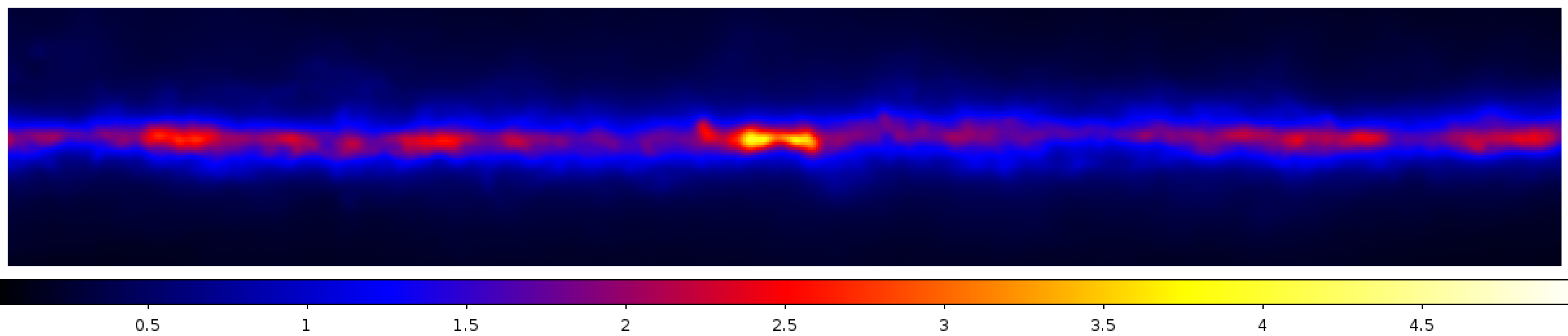
3.2. Make a model image with gtbin, gtexpcube2 and gtmodel

Next we want to make a model image (a.k.a an “expected counts image”) for the diffuse Galactic and isotropic emission. See here for information on these diffuse model components that are considered “background” for gamma-ray source analysis.

To get this image we need to run the following three Fermi ScienceTools in sequence:

• gtbin with the CCUBE option.
• gtexpcube2
• gtmodel

First we need to describe the model, which we do in the XML file diffuse_model.xml:

<?xml version="1.0" ?>
<source_library title="source library">

<!-- Diffuse Sources -->
<source name="gal_2yearp7v6_v0" type="DiffuseSource">
	<spectrum type="PowerLaw">
		<parameter free="1" max="10" min="0" name="Prefactor" scale="1" value="1"/>
		<parameter free="0" max="1" min="-1" name="Index" scale="1.0" value="0"/>
		<parameter free="0" max="2e2" min="5e1" name="Scale" scale="1.0" value="1e2"/>
	</spectrum>
	<spatialModel file="gal_2yearp7v6_v0.fits" type="MapCubeFunction">
		<parameter free="0" max="1e3" min="1e-3" name="Normalization" scale="1.0" value="1.0"/>
	</spatialModel>
</source>
<source name="iso_p7v6source" type="DiffuseSource">
	<spectrum file="iso_p7v6source.txt" type="FileFunction">
		<parameter free="1" max="10" min="1e-2" name="Normalization" scale="1" value="1"/>
	</spectrum>
	<spatialModel type="ConstantValue">
		<parameter free="0" max="10.0" min="0.0" name="Value" scale="1.0" value="1.0"/>
	</spatialModel>
</source>

</source_library>

Next we create symbolic links to the diffuse model files that come with the Fermi Science tools software distribution so that the tools will find them:

ln -s $FERMI_DIR/refdata/fermi/galdiffuse/gal_2yearp7v6_v0.fits .
ln -s $FERMI_DIR/refdata/fermi/galdiffuse/iso_p7v6source.txt .

Now we can run the tools to compute exposure and the PSF-convolved model image using these commands:

$ gtbin evfile=gtmktime.fits scfile=../../spacecraft.fits outfile=count_cube.fits \
  algorithm=CCUBE ebinalg=LOG emin=10e3 emax=316e3 enumbins=8 \
  nxpix=600 nypix=100 binsz=0.1 coordsys=GAL \
  xref=0 yref=0 axisrot=0 proj=CAR

$ gtexpcube2 infile=gtltcube.fits cmap=none outfile=gtexpcube2.fits \
  irfs=P7SOURCE_V6 nxpix=1800 nypix=900 binsz=0.2 coordsys=GAL \
  xref=0 yref=0 axisrot=0 proj=AIT \
  emin=10e3 emax=316e3 enumbins=8 bincalc=EDGE

$ gtmodel srcmaps=count_cube.fits srcmdl=diffuse_model.xml \
  outfile=model_image.fits irfs=P7SOURCE_V6 \
  expcube=gtltcube.fits bexpmap=gtexpcube2.fits

On my machine gtbin takes 5 seconds, gtexpcube2 takes 1 minute and gtmodel takes 5 minutes.

Note

Exercise: Inspect the generated files with ftlist and ds9 to see what they contain.

Consult the official Fermi LAT Binned Likelihood Tutorial analysis thread for detailed information.