Aperture Lightcurve
Computing the aperture lightcurve
In this section of the tutorial we will learn how to generate an aperture lightcurve from Fermi/LAT.
There are two different kinds of lightcurves that can be computed from Fermi/LAT observations: using likelihood analysis on each of the lightcurve bins, or aperture analysis. The likelihood analysis leads to a better sensitivity and the ability to obtain background-substracted flux lightcurves, but is model-dependent and very computationally intensive, especially for longer periods of time. Aperture lightcurve generation, on the other hand, is less computationally demanding and provides a model-independent estimate of the variability of a given source. However, there is no way to do an estimation of the background, so it should not be used to estimate the source’s flux.
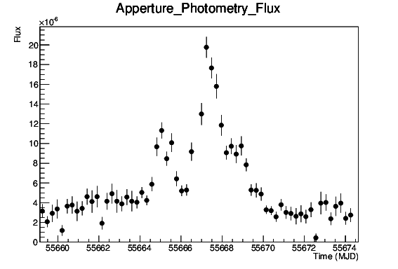
Here we will compute the aperture lightcurve of the remarkable April 2011 flare from the Crab Nebula. The Crab Nebula has been used for decades as the standard candle in High Energy Astrophysics, as it is bright and expected to have a constant flux. However, Fermi/LAT discovered that its flux is far from constant, exhibiting flux changes of a factor of 10 or more over just a few hours. The astrophysical process behind these flares is still unkown.
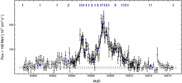
Fermi/LAT lightcurve of the April 2011 Crab Nebula flare as published in Buehler et al. (2012), ApJ 749, 26
In this tutorial we assume that you have already installed and initialized the Fermi Science Tools as well as enrico.
Change directory to where you have extracted the excercise data files and enter the lightcurve directory. You can explore the data selection applied to the event file with gtvcut command.
Generate an configuration file for this observation with the command:
$ enrico_config crab.conf
and enter the name and coordinates of the source (you will find them in the data selection cuts shown with gtvcut). For the aperture lightcurve, the model and ROI size parameters are not used, so leave them to their default values. Finally, select the initial and final analysis times as given in the server query file.
You can the edit the file crab.conf to check the parameters. In addition to the target, space, file, and time categories, the AppLC configuration category includes the values used by enrico when creating the aperture lightcurve. Use the NLCbin parameter to set the number of bins desired in the lightcurve between tmin and tmax. Given that the total selection time in the photon file is 16 days, 32 bins will result in a bin width of 12 hours, and 64 bins in a bin width of 24 hours. You can try different bin widths to check which one yields the most informative lightcurve, taking into account that shorter time bin widths will result in larger uncertainties.
During these observations the survey mode of the Fermi observatory was changed in favour of pointed observations towards the Crab Nebula. For this reason, one of the filter options in crab.conf (ABS(ROCK_ANGLE)<52) should be removed as it is related to the survey mode spacecraft rocking. The resulting filter expression in [analysis]/filter should be:
[analysis]
    filter = DATA_QUAL==1&&LAT_CONFIG==1
Finally, run the aperture lightcurve enrico script:
$ enrico_applc crab.conf
This scrip will run the following tasks:
- gtselect : Select the events from the input FT1 file.
- gtmktime : Compute good time intervals based on spacecraft pointing and SAA position.
- gtbin : Bin the data into a lightcurve.
- gtexposure : Compute the exposure (effective area*observation time) for each of the bins.
- From the results of gtbin and gtexposure, lightcurve plots are generated in the AppertureLightcurve directory.
The resulting aperture lightcurve will be saved in AppertureLightcurve/AppLC.eps, and should reproduce the two peaks shown in Buehler et al. (2012) as seen in the following example: